Analysis of NanoString CosMx data

This tutorial shows how you can analyse NanoString CosMx data with SPArrOW. The dataset used in this tutorial is the colon adenocarcinoma from https://doi.org/10.1038/s41467-025-64292-3.

%load_ext autoreload
%autoreload 2

import os
import uuid
import tempfile

import dask.array as da
from dask_image.imread import imread
from dask.dataframe import read_parquet

import spatialdata as sd
from spatialdata import bounding_box_query
from spatialdata.models import Image2DModel, PointsModel

import scanpy as sc
import sparrow as sp
from sparrow.utils._keys import _ANNOTATION_KEY

# change this path. It is the directory where the spatialdata .zarr will be saved.
# OUTPUT_DIR = tempfile.gettempdir()
OUTPUT_DIR = "data/results"

# you can choose any name for your zarr file
ZARR_PATH = os.path.join(OUTPUT_DIR, f"sdata_{uuid.uuid4()}.zarr")
ZARR_SUBSET_PATH = os.path.join(OUTPUT_DIR, f"sdata_subset_{uuid.uuid4()}.zarr")

PATH_IMAGE = "data/cosmx_coad/DAPI.tif"
PATH_COORDINATES = "data/cosmx_coad/transcripts/tx_file.parquet"
# PATH_MARKER_GENES = registry.fetch("data/cosmx_coad/marker_genes.csv")
PATH_MARKER_GENES = "data/cosmx_coad/marker_genes.csv"

1. Read in the data

The first step of the SPArrOW pipeline includes reading in the raw data. This, minimally, includes the stained image(s) and the transcript locations which should be aligned. For CosMx data, it could be possible that the download DAPI image and the transcripts are not yet aligned.

The example dataset for this notebook will be downloaded and cached using pooch via sparrow.dataset.registry. This dataset still needs to be aligned. To save time and computational resources, the tutorial will use a small subset.

The transcript location file is expected to be a parquet file. The image is then read in to a SpatialData object (see https://spatialdata.scverse.org/en/latest/ for more information). As the Spatial datasets are often larger-than memory, a path to where all data will be stored is asked.

When working on GPU, it is advisable to define a client to avoid memory issues.

def load_full_dataset() -> sd.SpatialData:
    # Load the DAPI image and align the orientation with the transcripts
    dapi = imread(PATH_IMAGE)
    dapi = da.flip(dapi, axis=1).rechunk((1, 5_000, 5_000))
    
    # Load transcripts positions and align with the DAPI image
    transcripts = read_parquet(
        PATH_COORDINATES, 
        columns=["x_global_px", "y_global_px", "target"]
    ).rename(columns={"target": "gene"})
    
    transcripts["y_global_px"] += 4255.90024432164 # Correct for minumum at zero
    
    # Create a SpatialData object to store all results
    sdata = sd.SpatialData(
        images={"raw_image": Image2DModel.parse(dapi)}, 
        points={"transcripts": PointsModel.parse(transcripts, coordinates={"x": "x_global_px", "y": "y_global_px"})}
    )
    
    sdata.write(ZARR_PATH)
    return sdata

def subset_full_dataset(sdata: sd.SpatialData) -> sd.SpatialData:

    sdata = bounding_box_query(
        sdata, 
        axes=[ "x", "y" ], 
        min_coordinate=[0,  0], 
        max_coordinate=[21_000, 21_000],  
        target_coordinate_system="global" 
    )

    sdata.write(ZARR_SUBSET_PATH)
    sdata = sd.read_zarr(ZARR_SUBSET_PATH)
    return sdata

%%time

# from sparrow.datasets.registry import get_registry

# registry = get_registry()
# path_image = registry.fetch("https://bj21400.api.aliyunfile.com/v2/redirect?id=e180d9b6a5034b2d968b85bf3e711af61763121359560203062")
# path_coordinates = registry.fetch("transcriptomics/resolve/mouse/20272_slide1_A1-1_results.txt")

sdata = load_full_dataset()
sdata = subset_full_dataset(sdata)

# sdata = registry.fetch("https://bj21400.api.aliyunfile.com/v2/redirect?id=e180d9b6a5034b2d968b85bf3e711af61763121359560203062")

INFO     no axes information specified in the object, setting `dims` to: ('c', 'y', 'x')
INFO     The Zarr backing store has been changed from None the new file path:                                      
         data/results/sdata_bd8f4797-b623-49b2-95d2-9da6ae13abda.zarr
INFO     The Zarr backing store has been changed from None the new file path:                                      
         data/results/sdata_subset_00d8899b-799e-49bd-97f9-abf9f491f648.zarr
CPU times: user 28min 14s, sys: 7min 51s, total: 36min 6s
Wall time: 1min 58s

sdata = sd.read_zarr("data/cosmx_coad/sdata_subset_2.zarr")

sdata = sd.SpatialData(
    images={"raw_image": sdata["raw_image"]},
    points={"transcripts": sdata["transcripts"]}
)

sdata.write(ZARR_SUBSET_PATH)
sdata

INFO     The SpatialData object is not self-contained (i.e. it contains some elements that are Dask-backed from    
         locations outside data/results/sdata_subset_a91f25c8-28a4-4196-82bf-97cfa59415bb.zarr). Please see the    
         documentation of `is_self_contained()` to understand the implications of working with SpatialData objects 
         that are not self-contained.                                                                              
INFO     The Zarr backing store has been changed from None the new file path:                                      
         data/results/sdata_subset_a91f25c8-28a4-4196-82bf-97cfa59415bb.zarr

SpatialData object, with associated Zarr store: /srv/scratch/xanderw/sparrow_cosmx/data/results/sdata_subset_a91f25c8-28a4-4196-82bf-97cfa59415bb.zarr
├── Images
│     └── 'raw_image': DataArray[cyx] (1, 21000, 21000)
└── Points
      └── 'transcripts': DataFrame with shape: (<Delayed>, 3) (2D points)
with coordinate systems:
    ▸ 'global', with elements:
        raw_image (Images), transcripts (Points)
with the following Dask-backed elements not being self-contained:
    ▸ raw_image: /srv/scratch/xanderw/sparrow_cosmx/data/cosmx_coad/sdata_subset_2.zarr/images/raw_image

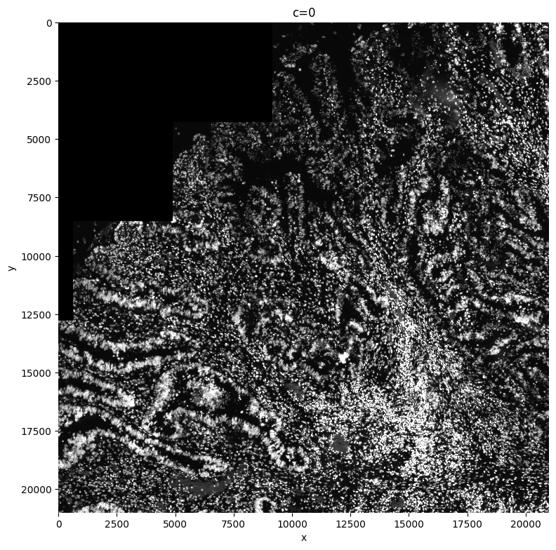
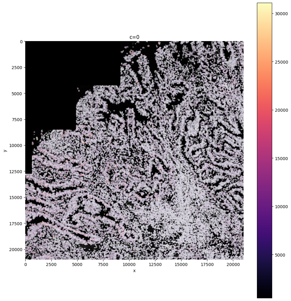
1.1 Plot the image(s)

sp.pl.plot_image(sdata, img_layer="raw_image", figsize=(8, 8))

2. Processing the image(s)

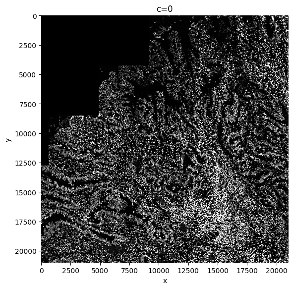
min-max filtering and contrast enhancing

The second step of preprocessing the data includes a couple of steps:

• A min-max filter can be added. The goal of this function is to substract background noise, and make the borders of the nuclei/cells cleaner, plus it will delete the occasional debris. If you take the size too small, smaller than the size of your nuclei, the function will create donuts, with black spots in the center of your cells. If the size of the min-max filter is chosen too big, not enough background is substracted, so a tradeoff should be made. This might need some finetuning. Bigger for whole cells. Adapt this parameter to make sure you delete debris and HALO’s.

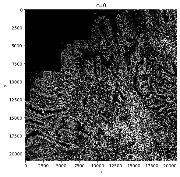
• We recommend to perform contrast enhancing on your image. SPArrOW does this by using histogram equalization (CLAHE function). The amount of correction needed can be decided by adapting the contrast_clip value. If the image is already quite bright, 3.5 might be a good starting value. For dark images, you can go up to 10 or even more. Make sure at the end the whole image is evenly illuminated and no cells are dark in the background.

In every cleaning step, a new image is created and written to disk, that is then used as an input for the next step.

%%time

sdata = sp.im.min_max_filtering(
    sdata=sdata, 
    img_layer="raw_image", 
    output_layer="min_max_filtered_171", 
    size_min_max_filter=171, 
    overwrite=True
)
sp.pl.plot_image(sdata, img_layer="min_max_filtered_171", figsize=(6, 6))

sdata = sp.im.enhance_contrast(
    sdata=sdata, 
    img_layer="min_max_filtered_171", 
    output_layer="clahe_50", 
    contrast_clip=50, 
    chunks=20000, 
    overwrite=True, 
)
sp.pl.plot_image(sdata, img_layer="clahe_50", figsize=(6, 6))

CPU times: user 1min 42s, sys: 41.5 s, total: 2min 24s
Wall time: 1min 39s

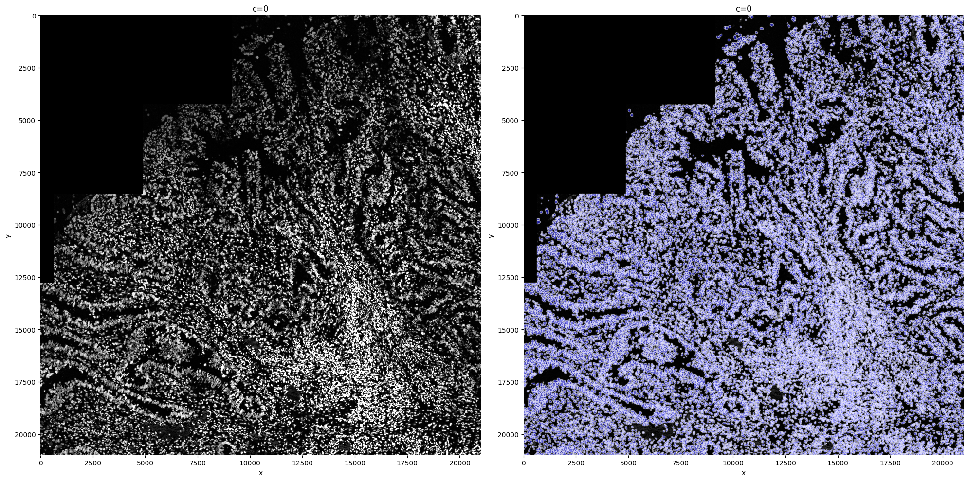
3. Segmenting the image

For the segmentation, we here show an example on how to use cellpose, a deep learning network based on a UNET architecture. This is a great tool , because it segments both nuclei and whole cells.

Multiple paramters need to be given as an input to the cellpose algorithm. We recommend tuning for the optimal segmentation quality.

• diameter: Includes an estimate of the diameter of a nucleus. If put to none, cellpose will do the estimation by himself, but this estimation might take longer than the actual segmentation, and if often far off. Input is in pixels. This of course is tissue and method dependent. You can run the algorthim on a small piece (I[0:1000,0:1000] for example), to get an estimate of the size. However, this estimate isn’t always accurate. So check the quality at the end. If you see all nuclei/cells are estimated too small, enlarge this parameter.

• device: Defines the device you want to work on, if you only have cpu, you can skip this input parameter. If only having CPU, please tune the parameters on a small subset, and then make it to the big one. This might take a while for large images, but it should work.

• flow_threshold: Indicates something about the shape of the masks, if you increase it, more masks with less round shapes will be accepted. A recommended range is 0.6 and 0.95, depending on the cell shapes. Higher is less round. Lower it if you start segmenting artefacts, up it if you miss non-round shaped cells.

• mask_threshold: Indicates how many of the possible masks are kept. Making it smaller (up to -6), will give you more masks, bigger is less masks (up to 0). Be careful, you can oversegment: always check the quality

• min_size: Indicates the minimal size of a nucleus.

%%time

sdata = sp.im.segment(
    sdata=sdata,
    img_layer="clahe_50",
    output_labels_layer="segmentation_mask_75_095_m6",
    output_shapes_layer="segmentation_mask_boundaries_75_095_m6",
    device="cuda",
    min_size=80,
    flow_threshold=0.95,
    diameter=75,
    cellprob_threshold=-6,
    chunks=2048,
    depth=100,
    overwrite=True,
)

sp.pl.segment(sdata=sdata, img_layer="clahe_50", shapes_layer="segmentation_mask_boundaries_75_095_m6")

CPU times: user 50min 24s, sys: 2min 55s, total: 53min 19s
Wall time: 6min 48s

4. Allocating the transcripts

4.1 Creating the count matrix

In this step we allocate the transcripts to the correct cell. This allocation step creates the count matrix, saved in an anndata object that is reachable by typing sdata.table

sdata = sp.tb.allocate(
    sdata=sdata,
    labels_layer="segmentation_mask_75_095_m6",
    points_layer="transcripts",
    output_layer="table_transcriptomics",
    overwrite=True,
)

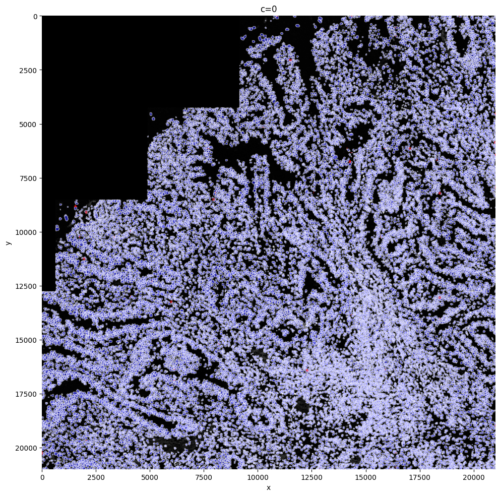
In this step, there might be semgented entities that do not contain any transcripts. These entities are filtered out of the semgentation_mask_boundaries shapes layer and aren’t added to the anndata. Instead these shapes are now saved in filtered_semgentation_segmentation_mask_boundaries. It is possible to visualize these entities on the image with red borders, by making use of the shapes_layer_filtered parameter. As you can see, in this case, 110 entities were filtered. This will be very dataset dependent. When there are regions with necrosis for example, this number will be way higher. Visualizing these cells shows clearly on plots that those cells weren’t missed with segmentation, but were missed becasue of no transcripts measured, an issue? SPArrOW cannot solve.

sp.pl.plot_shapes(
    sdata,
    img_layer="clahe_50",
    shapes_layer="segmentation_mask_boundaries_75_095_m6",
    shapes_layer_filtered="filtered_segmentation_segmentation_mask_boundaries_75_095_m6",
)

4.2 Transcript quality plot

After we have created the anndata object, we control the transcript quality.

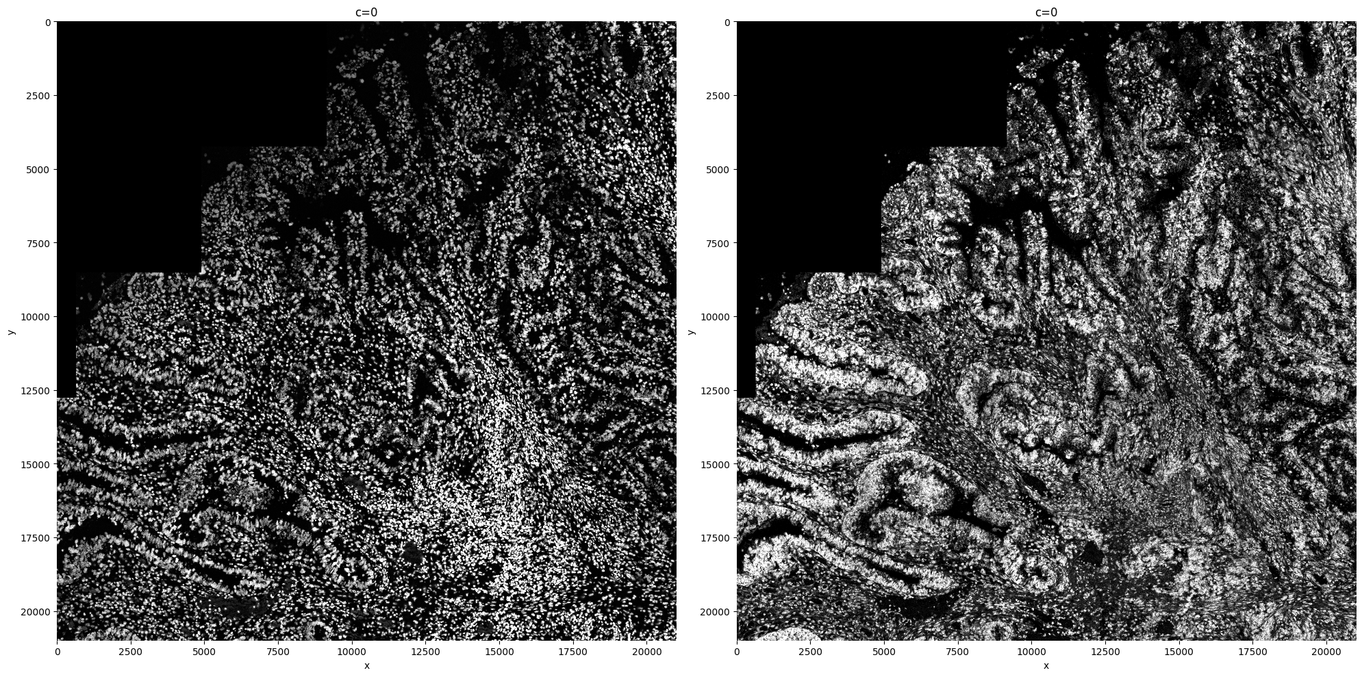
First we create a plot to check if the transcript density is similar across the whole tissue. If this is not the case, it can have multiple reasons. Most likely, there will be regions in which the transcript pick-up was less succesfull. Also gene panel choices can influence this plot.

sdata = sp.im.transcript_density(
    sdata,
    img_layer="clahe_50",
    points_layer="transcripts",
    output_layer="transcript_density",
    overwrite=True,
)
sp.pl.transcript_density(sdata, img_layer=["clahe_50", "transcript_density"])

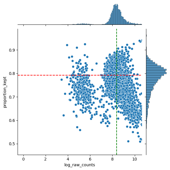
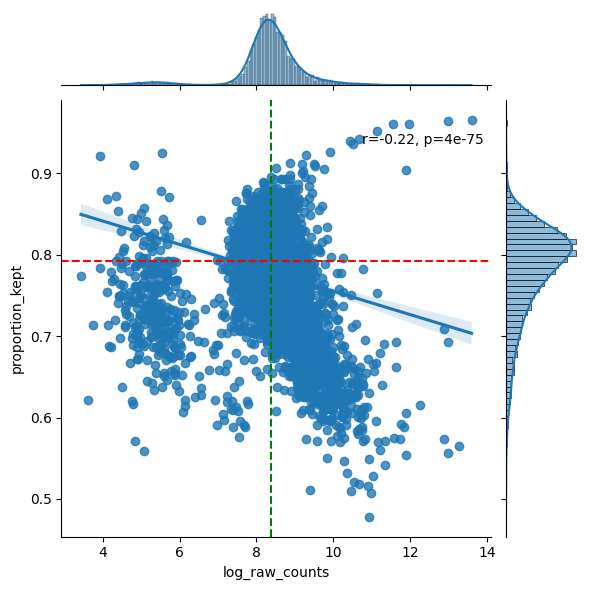
As not all of the image surface is segmented, there will be most likely transcripts that weren’t assigned to a cell. For sure in the case of nucleus segmentation (like this example), this will be the case.

In general, we hope to not lose any genes. So we hope there are no genes with low abundances and a low proportion kept. In general we see a downward trend. The more a gene is measured, the less it is located in cells (in ratio).

We also provide a table with the genes that are the least located in cells. If a lot of these genes are markers for the same celltype, the staining might be missing this celltype and you should for sure check this. However, it might also be the case that is celltype just has a lot of cytoplasm and you are only semgenting the nucleus.

filtered = sp.pl.analyse_genes_left_out(
    sdata,
    labels_layer="segmentation_mask_75_095_m6",
    table_layer="table_transcriptomics",
    points_layer="transcripts",
)

---------------------------------------------------------------------------
AttributeError                            Traceback (most recent call last)
Cell In[12], line 1
----> 1 filtered = sp.pl.analyse_genes_left_out(
      2     sdata,
      3     labels_layer="segmentation_mask_75_095_m6",
      4     table_layer="table_transcriptomics",
      5     points_layer="transcripts",
      6 )

File /srv/scratch/xanderw/sparrow_cosmx/.venv/lib64/python3.11/site-packages/sparrow/plot/_transcripts.py:160, in analyse_genes_left_out(sdata, labels_layer, table_layer, points_layer, to_coordinate_system, counts_layer, name_x, name_y, name_gene_column, output)
    158 plt.axvline(filtered[f"log_{_RAW_COUNTS_KEY}"].median(), color="green", linestyle="dashed")
    159 plt.axhline(filtered["proportion_kept"].median(), color="red", linestyle="dashed")
--> 160 plt.ax_marg_x.axvline(x=filtered[f"log_{_RAW_COUNTS_KEY}"].median(), color='green')
    161 plt.ax_marg_y.axhline(y=filtered["proportion_kept"].median(), color="red")
    163 if output:

AttributeError: module 'matplotlib.pyplot' has no attribute 'ax_marg_x'

5. Preprocess adata

5.1 Filtering and Normalization

The anndata object is now processed:

• calculate QC metrics

• filter cells with less then 10 gene counts and genes with less then 5 cells (adaptations possible by adapting the function). These filtered cells are again filtered out of the shapes layer and the anndata obejct and saved in an extra shapes layer.

• Normalization: For small gene panel (<500), we recommend to normalize the data based on the size of the segmented object (size_norm=True). For transcriptome-wide methods, we recommend standard library size normalization (size_norm=False).

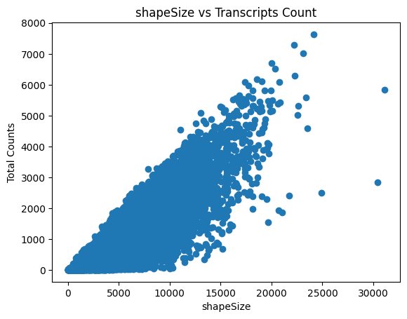
The last plot shows the size of the nucleus related to the counts. When working with whole cells, if there are some really big cells with really low counts, they are probably not real cells and you should filter based on max size.

# Remove control genes
ctrl_genes = [gene for gene in sdata['table_transcriptomics'].var_names if "SystemControl" in gene]
sdata["table_transcriptomics"] = sdata["table_transcriptomics"][:, ~sdata["table_transcriptomics"].var_names.isin(ctrl_genes)]

# Perform preprocessing.
sdata = sp.tb.preprocess_transcriptomics(
    sdata,
    labels_layer="segmentation_mask_75_095_m6",
    table_layer="table_transcriptomics",
    output_layer="table_transcriptomics_preprocessed",  # write results to a new slot, we could also write to the same slot (when passing overwrite==True).
    min_counts=10,
    min_cells=5,
    size_norm=False,
    highly_variable_genes=False,
    n_comps=50,
    overwrite=True,
)

The raw counts are saved in sdata.tables['table_transcriptomics_preprocessed'].layers['raw_counts']. The size normalized data in .raw.

sdata.tables["table_transcriptomics_preprocessed"].raw.to_adata().to_df()

	A1BG	A2M	AAAS	AAK1	AAMP	AARS1	AASS	AATK	ABAT	ABCA1	...	ZNF804A	ZNRF1	ZNRF2	ZNRF3	ZP3	ZSWIM6	ZWINT	ZYG11B	ZYX	ZZZ3
cells
138_segmentation_mask_75_095_m6_faab4c83	0.000000	0.000000	0.0	0.0	1.074364	0.0	0.000000	0.000000	0.000000	0.0	...	0.0	0.0	0.000000	0.000000	0.0	0.000000	0.0	0.000000	0.000000	0.000000
144_segmentation_mask_75_095_m6_faab4c83	0.000000	0.000000	0.0	0.0	0.827713	0.0	0.000000	0.000000	0.000000	0.0	...	0.0	0.0	0.000000	0.000000	0.0	0.000000	0.0	0.000000	0.827713	0.000000
152_segmentation_mask_75_095_m6_faab4c83	0.000000	0.550809	0.0	0.0	0.000000	0.0	0.000000	0.000000	0.550809	0.0	...	0.0	0.0	0.000000	0.903939	0.0	0.000000	0.0	0.000000	0.000000	0.000000
153_segmentation_mask_75_095_m6_faab4c83	0.000000	0.000000	0.0	0.0	0.000000	0.0	0.000000	0.000000	0.000000	0.0	...	0.0	0.0	0.000000	0.842915	0.0	0.000000	0.0	0.000000	0.000000	0.000000
165_segmentation_mask_75_095_m6_faab4c83	0.225088	0.000000	0.0	0.0	0.000000	0.0	0.225088	0.000000	0.000000	0.0	...	0.0	0.0	0.225088	0.000000	0.0	0.225088	0.0	0.408704	0.000000	0.225088
...	...	...	...	...	...	...	...	...	...	...	...	...	...	...	...	...	...	...	...	...	...
91777_segmentation_mask_75_095_m6_faab4c83	0.000000	0.000000	0.0	0.0	0.000000	0.0	0.000000	0.000000	0.000000	0.0	...	0.0	0.0	0.000000	0.000000	0.0	0.000000	0.0	0.000000	1.037451	0.000000
91905_segmentation_mask_75_095_m6_faab4c83	0.000000	0.000000	0.0	0.0	0.000000	0.0	0.000000	0.000000	0.000000	0.0	...	0.0	0.0	0.458627	0.000000	0.0	0.000000	0.0	0.000000	0.458627	0.000000
92160_segmentation_mask_75_095_m6_faab4c83	0.990026	0.990026	0.0	0.0	0.000000	0.0	0.000000	0.000000	0.000000	0.0	...	0.0	0.0	0.000000	0.000000	0.0	0.000000	0.0	0.000000	0.000000	0.000000
92288_segmentation_mask_75_095_m6_faab4c83	0.000000	0.000000	0.0	0.0	0.000000	0.0	0.000000	0.000000	0.000000	0.0	...	0.0	0.0	0.000000	0.000000	0.0	0.000000	0.0	0.000000	0.000000	0.000000
92543_segmentation_mask_75_095_m6_faab4c83	1.343972	0.882578	0.0	0.0	0.000000	0.0	0.000000	0.882578	0.000000	0.0	...	0.0	0.0	0.000000	0.000000	0.0	0.000000	0.0	0.000000	0.000000	0.000000

33532 rows × 6195 columns

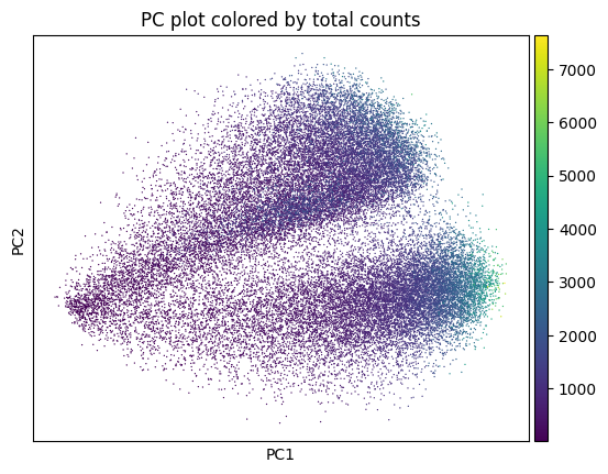
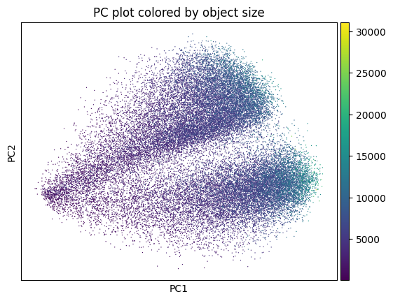
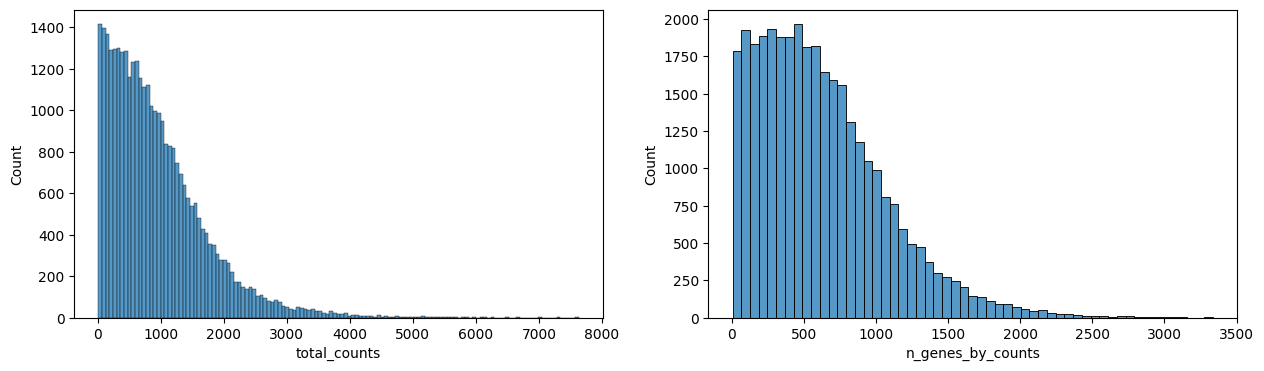
sp.pl.preprocess_transcriptomics(
    sdata,
    table_layer="table_transcriptomics_preprocessed",
)

sp.pl.plot_shapes(
    sdata,
    img_layer="clahe_50",
    table_layer="table_transcriptomics_preprocessed",
    column="total_counts",
    shapes_layer="segmentation_mask_boundaries_75_095_m6",
)

In this step you can filter cells based on their size: are you sure cells need to be bigger, or sure your cells can not be larger than X?

You can delete them with this function by defining min_size and max_size.

sdata = sp.tb.filter_on_size(
    sdata,
    labels_layer="segmentation_mask_75_095_m6",
    table_layer="table_transcriptomics_preprocessed",
    output_layer="table_transcriptomics_filter",
    min_size=500,
    max_size=100000,
    overwrite=True,
)

sp.pl.plot_shapes(
    sdata,
    img_layer="clahe_50",
    table_layer="table_transcriptomics_filter",
    column="shapeSize",
    shapes_layer="segmentation_mask_boundaries_75_095_m6",
)

You can see all filtered layers present in your sdata object under shapes

sdata

SpatialData object, with associated Zarr store: /srv/scratch/xanderw/sparrow_cosmx/data/results/sdata_subset_a91f25c8-28a4-4196-82bf-97cfa59415bb.zarr
├── Images
│     ├── 'clahe_50': DataArray[cyx] (1, 21000, 21000)
│     ├── 'min_max_filtered_171': DataArray[cyx] (1, 21000, 21000)
│     ├── 'raw_image': DataArray[cyx] (1, 21000, 21000)
│     └── 'transcript_density': DataArray[cyx] (1, 21000, 21000)
├── Labels
│     └── 'segmentation_mask_75_095_m6': DataArray[yx] (21000, 21000)
├── Points
│     └── 'transcripts': DataFrame with shape: (<Delayed>, 3) (2D points)
├── Shapes
│     ├── 'filtered_low_counts_segmentation_mask_boundaries_75_095_m6': GeoDataFrame shape: (274, 1) (2D shapes)
│     ├── 'filtered_segmentation_segmentation_mask_boundaries_75_095_m6': GeoDataFrame shape: (110, 1) (2D shapes)
│     ├── 'filtered_size_segmentation_mask_boundaries_75_095_m6': GeoDataFrame shape: (258, 1) (2D shapes)
│     └── 'segmentation_mask_boundaries_75_095_m6': GeoDataFrame shape: (33274, 1) (2D shapes)
└── Tables
      ├── 'table_transcriptomics': AnnData (33806, 6195)
      ├── 'table_transcriptomics_filter': AnnData (33274, 6195)
      └── 'table_transcriptomics_preprocessed': AnnData (33532, 6195)
with coordinate systems:
    ▸ 'global', with elements:
        clahe_50 (Images), min_max_filtered_171 (Images), raw_image (Images), transcript_density (Images), segmentation_mask_75_095_m6 (Labels), transcripts (Points), filtered_low_counts_segmentation_mask_boundaries_75_095_m6 (Shapes), filtered_segmentation_segmentation_mask_boundaries_75_095_m6 (Shapes), filtered_size_segmentation_mask_boundaries_75_095_m6 (Shapes), segmentation_mask_boundaries_75_095_m6 (Shapes)
with the following Dask-backed elements not being self-contained:
    ▸ raw_image: /srv/scratch/xanderw/sparrow_cosmx/data/cosmx_coad/sdata_subset_2.zarr/images/raw_image

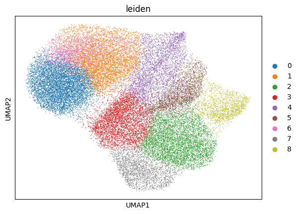
5.2 Clustering

This function performs the neighborhood analysis, the leiden clustering and the UMAP calculations using scanpy functions.

You need to define 2 parameters:

• the amount of PC’s used: choose something between 15-20 based on the plot of PC’s.

• The amount of neighbors used: Normally 35. Less neighbors means more spread, more means everything tighter, in general.

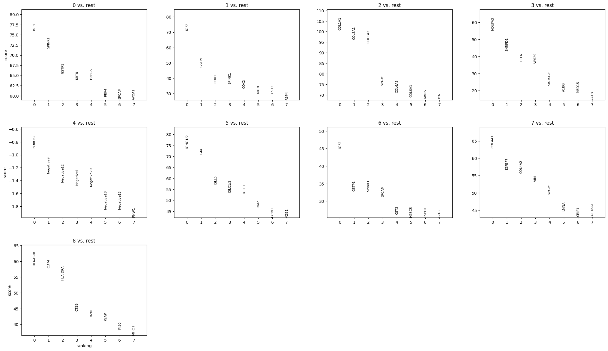
It returns the UMAP and marker gene list per cluster, that can be looked at for finding celltypes.

sdata = sp.tb.leiden(
    sdata,
    labels_layer="segmentation_mask_75_095_m6",
    table_layer="table_transcriptomics_filter",
    output_layer="table_transcriptomics_clustered",
    calculate_umap=True,
    calculate_neighbors=True,
    n_pcs=15,
    n_neighbors=35,
    resolution=0.8,
    rank_genes=True,
    key_added="leiden",
    overwrite=True,
)

sp.pl.cluster(
    sdata,
    table_layer="table_transcriptomics_clustered",
    key_added="leiden",
)

sp.pl.plot_shapes(
    sdata,
    img_layer="clahe_50",
    table_layer="table_transcriptomics_clustered",
    column="leiden",
    shapes_layer="segmentation_mask_boundaries_75_095_m6",
)

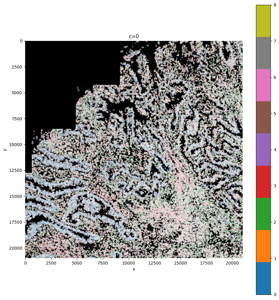
Here we reuse the plot_shapes function to actually plot a subfigure of our image with the cells colored based on the clustering.

6. Annotating the cells

Afte we created the count matrix, we are going to annotate the cells. SPArrOW has its own annotation algorithm, that starts fro m a marker gene list. It is an enrichment score algorithm, that compares the expression of marker genes in cells with a celltype weighted average. For this reason, the annotation happens iteratively.

The input marker gene list should be a csv file, with the marker genes in the rows and the celltypes in the columns. The weight given to a celltype/ marker gene combination should reflect the marker gene specifity of the gene to the celltype. binary inputs (zero for no marker, 1 for marker) are also accepted. A tutorial on how to create such marker genes lists from an atlas will follow.

A cell is annotated to be unknown if its score is lower than zero for all celltypes.

As the approach is iterative, the results of every step are shown.

sdata, celltypes_scored, celltypes_all = sp.tb.score_genes_iter(
    sdata,
    labels_layer="segmentation_mask_75_095_m6",
    table_layer="table_transcriptomics_clustered",
    output_layer="table_transcriptomics_score_genes_iter",
    path_marker_genes=PATH_MARKER_GENES,
    overwrite=True,
)

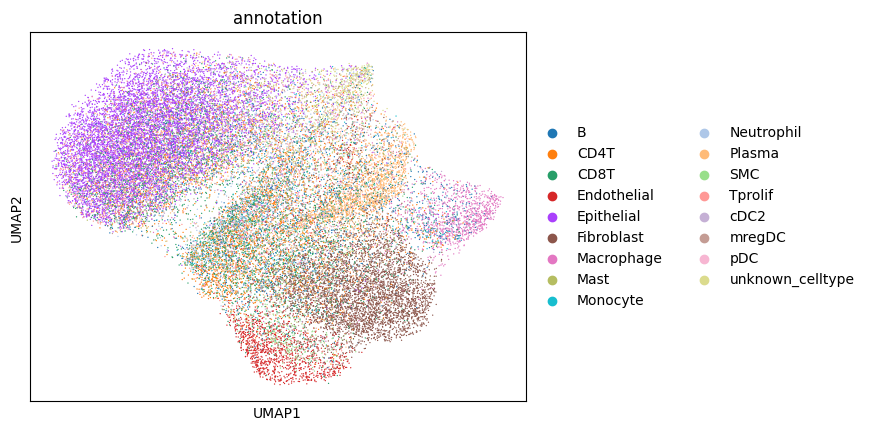
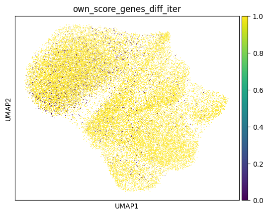
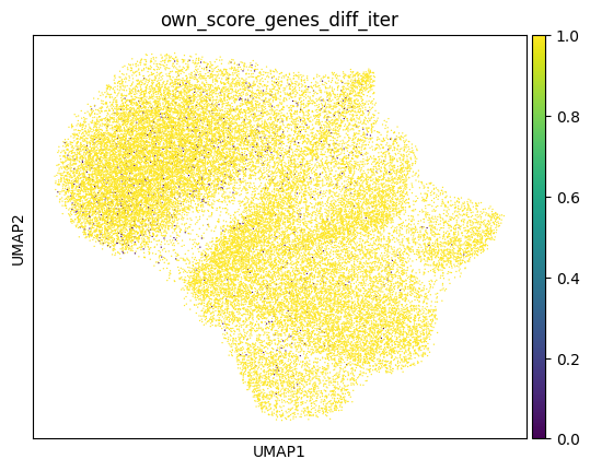
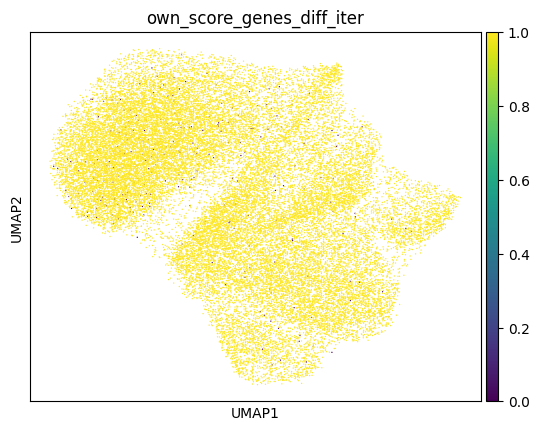
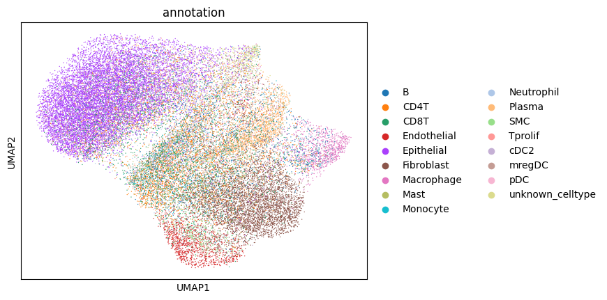
sc.pl.umap(sdata.tables["table_transcriptomics_score_genes_iter"], color=_ANNOTATION_KEY)

filtered_layers = [
    "filtered_segmentation_segmentation_mask_boundaries_75_095_m6",
    "filtered_low_counts_segmentation_mask_boundaries_75_095_m6",
    "filtered_size_segmentation_mask_boundaries_75_095_m6",
]

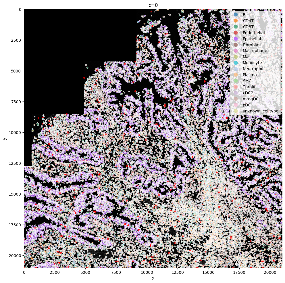
sp.pl.plot_shapes(
    sdata,
    column=_ANNOTATION_KEY,
    img_layer="clahe_50",
    table_layer="table_transcriptomics_score_genes_iter",
    shapes_layer="segmentation_mask_boundaries_75_095_m6",
    alpha=0.7,
    shapes_layer_filtered=filtered_layers,
)

Funcitonality from squidpy can be easily used from within SPArrOW, just run it on sdata.table. We impemented the neighborhood enrichment from scratch.

sdata = sp.tb.nhood_enrichment(
    sdata,
    labels_layer="segmentation_mask_75_095_m6",
    table_layer="table_transcriptomics_score_genes_iter",
    output_layer="table_transcriptomics_score_genes_enrichemnt",
    overwrite=True,
)

sp.pl.nhood_enrichment(
    sdata, table_layer="table_transcriptomics_score_genes_enrichemnt", celltype_column=_ANNOTATION_KEY
)

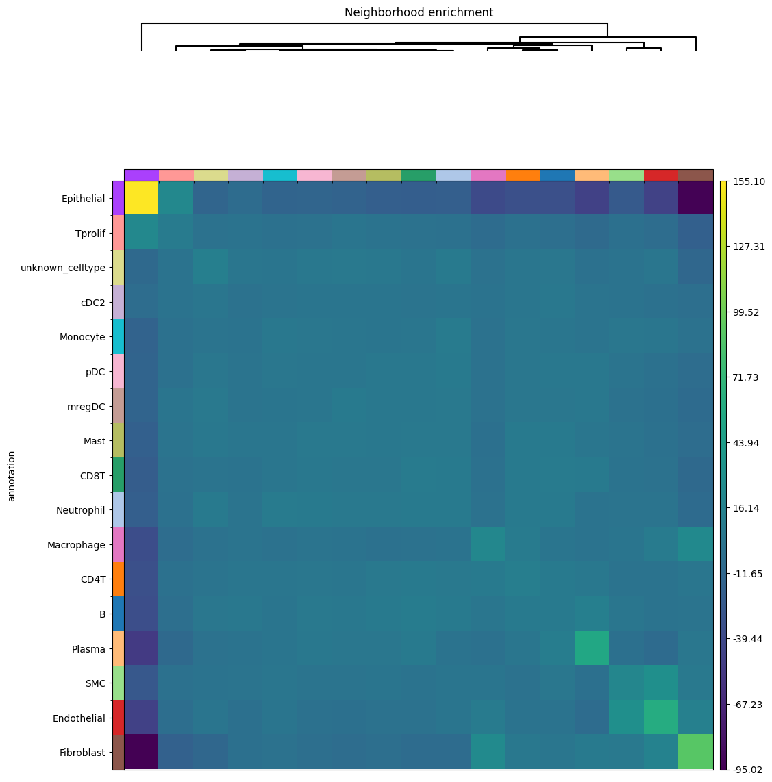
Use squidpy to see the enrichement between the different celltypes. For more info, see squidpy!