Analyzing MERFISH Data from the MERSCOPE Platform#
This tutorial illustrates how to analyze MERFISH spatial transcriptomics data using SPArrOW.
We will use a MERFISH mouse liver dataset generated on the Vizgen MERSCOPE platform, downloaded from https://info.vizgen.com/mouse-liver-data (accessed 2024-01-10).
Installation#
uv venv .venv_sparrow --python=3.12
source .venv_sparrow/bin/activate
uv pip install -e .
uv pip install jupyter
uv pip install rioxarray
uv pip install cellpose==3.1.1.1
uv pip install dask-cuda==24.12.0
uv pip install bokeh
%load_ext autoreload
%autoreload 2
import sparrow as sp
Download the data.#
from sparrow.datasets.registry import get_registry

registry = get_registry()

_ = registry.fetch("transcriptomics/vizgen/mouse/Liver1Slice1/images/mosaic_DAPI_z3.tif")
_ = registry.fetch("transcriptomics/vizgen/mouse/Liver1Slice1/images/mosaic_PolyT_z3.tif")
_ = registry.fetch("transcriptomics/vizgen/mouse/Liver1Slice1/images/micron_to_mosaic_pixel_transform.csv")
path_transcripts = registry.fetch("transcriptomics/vizgen/mouse/Liver1Slice1/detected_transcripts.csv")
Create the SpatialData object.#
import os
import tempfile

input_path = os.path.dirname(path_transcripts)
OUTPUT_DIR =  tempfile.gettempdir()

# This step can take around 20 minutes.
sdata = sp.io.merscope(
    path=input_path,
    to_coordinate_system="global",
    z_layers=[
        3,
    ],
    backend=None,
    transcripts=True,
    mosaic_images=True,
    do_3D=False,
    z_projection=False,
    image_models_kwargs={"scale_factors": None},
    output=os.path.join( OUTPUT_DIR, "sdata_merscope.zarr"),
    filter_gene_names=[ "blank" ],
)
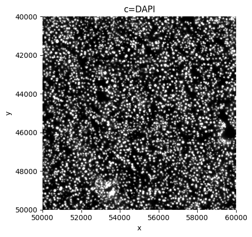
sp.pl.plot_shapes(
    sdata,
    img_layer=["mouse_Liver1Slice1_z3_global"],
    crd = [ 50000, 60000, 40000, 50000 ],
    channel="DAPI",
    figsize = (5,5),
     )
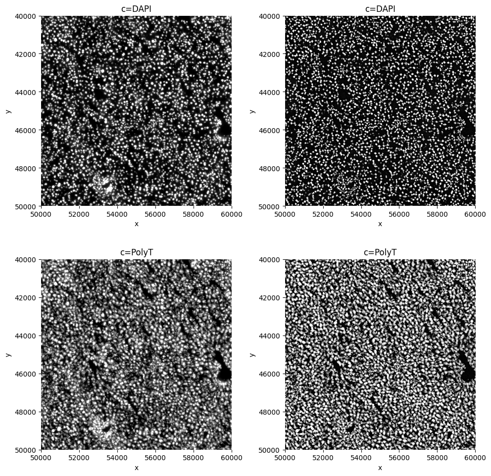
Preprocessing#
Note that we work on a crop for the rest of this tutorial.
sdata=sp.im.min_max_filtering(
    sdata,
    img_layer="mouse_Liver1Slice1_z3_global",
    output_layer="min_max_filtered",
    size_min_max_filter=[ 85, 135 ],
    crd = [ 50000, 60000, 40000, 50000 ],
    overwrite=True,
      )
sdata=sp.im.enhance_contrast(
    sdata,
    img_layer="min_max_filtered",
    output_layer="clahe",
    contrast_clip=[13.5, 18.5 ],
    crd = [ 50000, 60000, 40000, 50000 ],
    overwrite=True,
      )
sp.pl.plot_shapes(
    sdata,
    img_layer=["mouse_Liver1Slice1_z3_global", "clahe"],
    crd = [ 50000, 60000, 40000, 50000 ],
    figsize = (10,10),
    )
Segmentation#
sdata[ "clahe" ].c.data
array(['DAPI', 'PolyT'], dtype='<U5')
# rechunk on disk

from spatialdata.transformations import get_transformation

sdata = sp.im.add_image_layer(
    sdata,
    arr =sdata[ "clahe" ].data.rechunk( 4096 ),
    transformations=get_transformation( sdata[ "clahe"], get_all=True ),
    output_layer = "clahe",
    c_coords=sdata[ "clahe" ].c.data,
    overwrite=True,
     )
import torch
from dask.distributed import Client, LocalCluster

if torch.cuda.is_available():
    from dask_cuda import LocalCUDACluster  # pip install dask-cuda

    # One worker per GPU; each worker will be pinned to a single GPU.
    cluster = LocalCUDACluster(
        CUDA_VISIBLE_DEVICES=[0],  # or [0,1],...etc
        n_workers=1,  # 2 if [0,1],...etc
        threads_per_worker=1,
        memory_limit="32GB",
        local_directory=os.environ.get( "TMPDIR" ),
    )
else:
    # cpu/mps fall back
    from dask.distributed import LocalCluster

    cluster = LocalCluster(
        n_workers=1
        if torch.backends.mps.is_available()
        else 8,  # If mps/cuda device available, it is better to increase chunk size to maximal value that fits on the gpu, and set n_workers to 1.
        # For this dummy example, we only have one chunk, so setting n_workers>1, has no effect.
        threads_per_worker=1,
        memory_limit="32GB",
        local_directory=os.environ.get( "TMPDIR" ),
    )

client = Client(cluster)

print(client.dashboard_link)
http://127.0.0.1:36989/status
from sparrow.image._image import _get_spatial_element

se = _get_spatial_element( sdata, layer = "clahe" )

sdata = sp.im.segment(
    sdata,
    img_layer="clahe",
    depth=200,
    model=sp.im.cellpose_callable,
    # parameters that will be passed to the callable sp.im.cellpose
    pretrained_model = "cyto3",
    diameter=100,
    flow_threshold=0.85,
    cellprob_threshold=-4,
    channels = [ se.c.data.tolist().index("PolyT" )+1, se.c.data.tolist().index("DAPI" )+1 ],
    output_labels_layer="segmentation_mask_crop",
    output_shapes_layer="segmentation_mask_boundaries_crop",
    crd= [50000, 60000, 40000, 50000],  # region to segment [x_min, xmax, y_min, y_max],
    overwrite=True,
)

client.close()
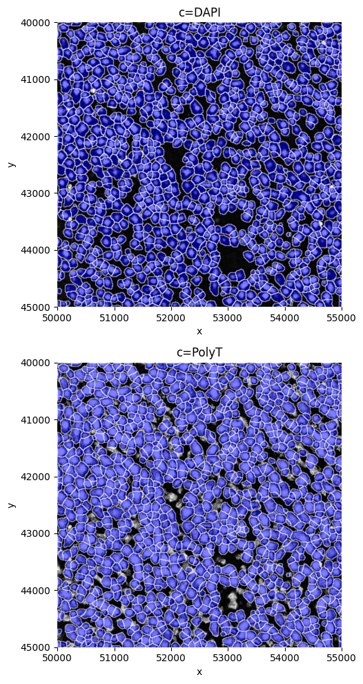
sp.pl.plot_shapes(
    sdata,
    shapes_layer="segmentation_mask_boundaries_crop",
    img_layer=["clahe"],
    crd = [ 50000, 55000, 40000, 45000 ],
    figsize=( 10,10 ),
    )
Create the AnnData table#
sdata = sp.tb.allocate(
    sdata=sdata,
    labels_layer="segmentation_mask_crop",
    points_layer="transcripts_global",
    output_layer="table_transcriptomics_crop",
    update_shapes_layers=False,
    overwrite=True,
)
sp.pl.sanity(
    sdata,
    img_layer="clahe",
    shapes_layer = "segmentation_mask_boundaries_crop",
    points_layer= "transcripts_global",
    plot_cell_number=True,
    gene="Vwf",
    crd = [ 50500, 50500+500, 41000, 41500 ],
    figsize=(5,5),
)
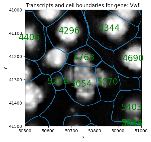
# Look-up a the number of transcripts for the Vwf gene in a cell shown above (using the cell ID),
# it should be the same number as transcripts plotted above.

sdata[ "table_transcriptomics_crop" ][sdata[ "table_transcriptomics_crop" ].obs[ "cell_ID" ] == 4296].to_df()["Vwf"]
cells
4296_segmentation_mask_crop_e0acaceb    1
Name: Vwf, dtype: uint32
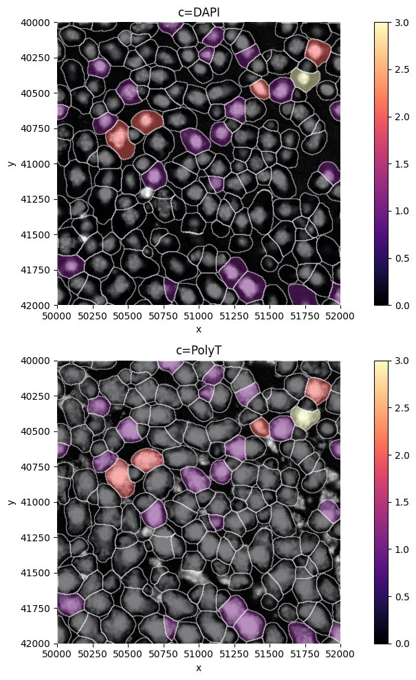
Visualize gene expression#
sp.pl.plot_shapes(
    sdata,
    img_layer="clahe",
    shapes_layer="segmentation_mask_boundaries_crop",
    figsize=( 10,10 ),
    crd = [  50000, 52000, 40000, 42000  ],
    table_layer="table_transcriptomics_crop",
    column = "Vwf",
      )
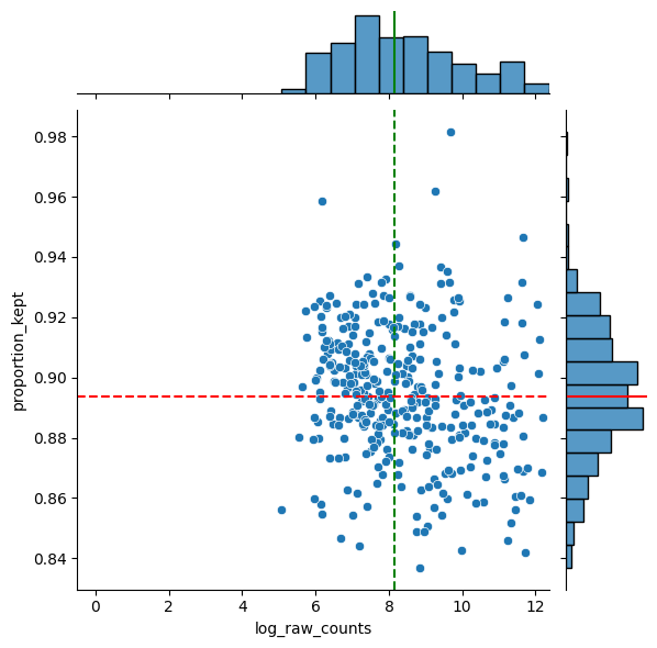
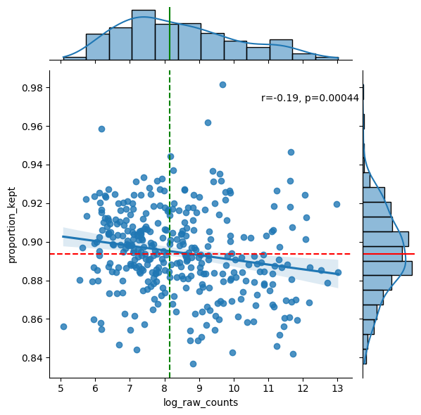
df = sp.pl.analyse_genes_left_out(
    sdata,
    labels_layer="segmentation_mask_crop",
    table_layer="table_transcriptomics_crop",
    points_layer="transcripts_global",
)
Preprocess the AnnData table#
# Perform preprocessing.
sdata = sp.tb.preprocess_transcriptomics(
    sdata,
    labels_layer="segmentation_mask_crop",
    table_layer="table_transcriptomics_crop",
    output_layer="table_transcriptomics_preprocessed_crop",  # write results to a new slot, we could also write to the same slot (when passing overwrite==True).
    min_counts=10,
    min_cells=5,
    size_norm=True,
    n_comps=50,
    overwrite=True,
    update_shapes_layers=False,
)
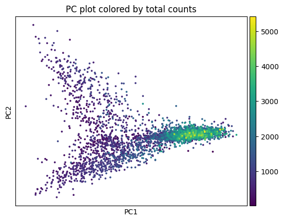
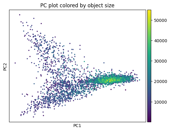
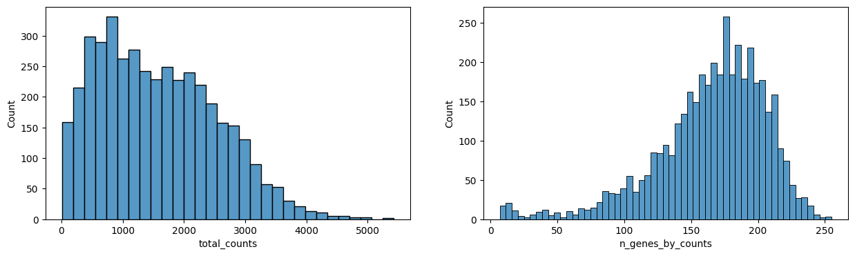
sp.pl.preprocess_transcriptomics(
    sdata,
    table_layer="table_transcriptomics_preprocessed_crop",
)
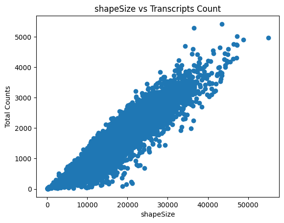
sdata = sp.tb.filter_on_size(
    sdata,
    labels_layer="segmentation_mask_crop",
    table_layer="table_transcriptomics_preprocessed_crop",
    output_layer="table_transcriptomics_filter_crop",
    min_size=500,
    max_size=100000,
    update_shapes_layers=False,
    overwrite=True,
)
Leiden clustering#
import scanpy as sc
sdata = sp.tb.leiden(
sdata,
labels_layer="segmentation_mask_crop",
table_layer="table_transcriptomics_filter_crop",
output_layer="table_transcriptomics_clustered_crop",
calculate_umap=True,
calculate_neighbors=True,
n_pcs=17,
n_neighbors=35,
resolution=1.0,
rank_genes=True,
key_added="leiden",
overwrite=True,
)
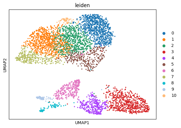
sc.pl.umap(sdata.tables["table_transcriptomics_clustered_crop"], color=["leiden"], show=True)
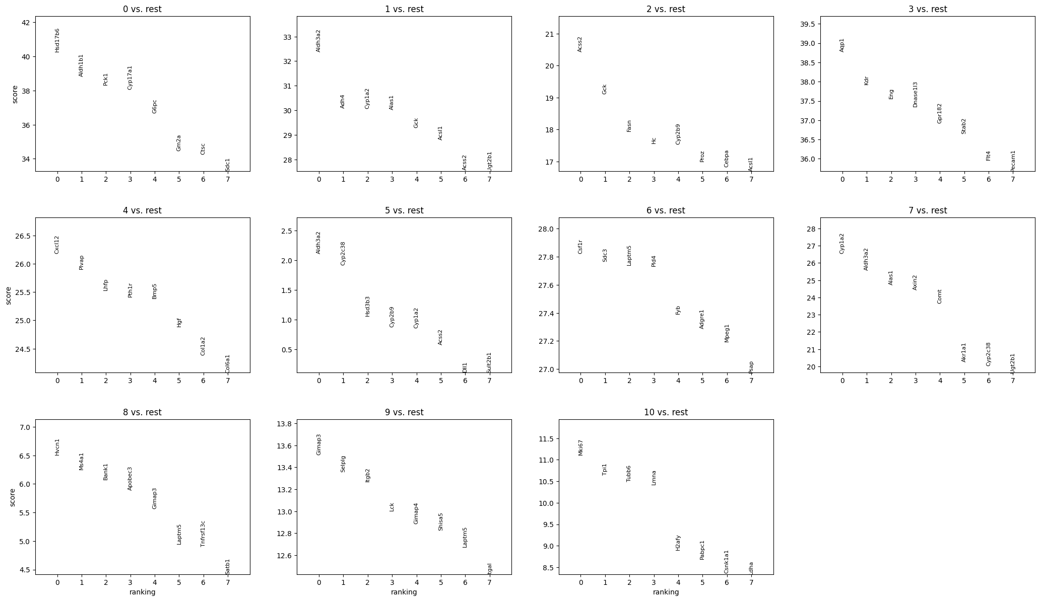
sc.pl.rank_genes_groups(sdata.tables["table_transcriptomics_clustered_crop"], n_genes=8, sharey=False, show=True)
sdata[ "table_transcriptomics_clustered_crop" ].obs[ "leiden" ].head()
cells
149_segmentation_mask_crop_e0acaceb    7
181_segmentation_mask_crop_e0acaceb    7
229_segmentation_mask_crop_e0acaceb    1
264_segmentation_mask_crop_e0acaceb    1
293_segmentation_mask_crop_e0acaceb    3
Name: leiden, dtype: category
Categories (11, int64): [0, 1, 2, 3, ..., 7, 8, 9, 10]
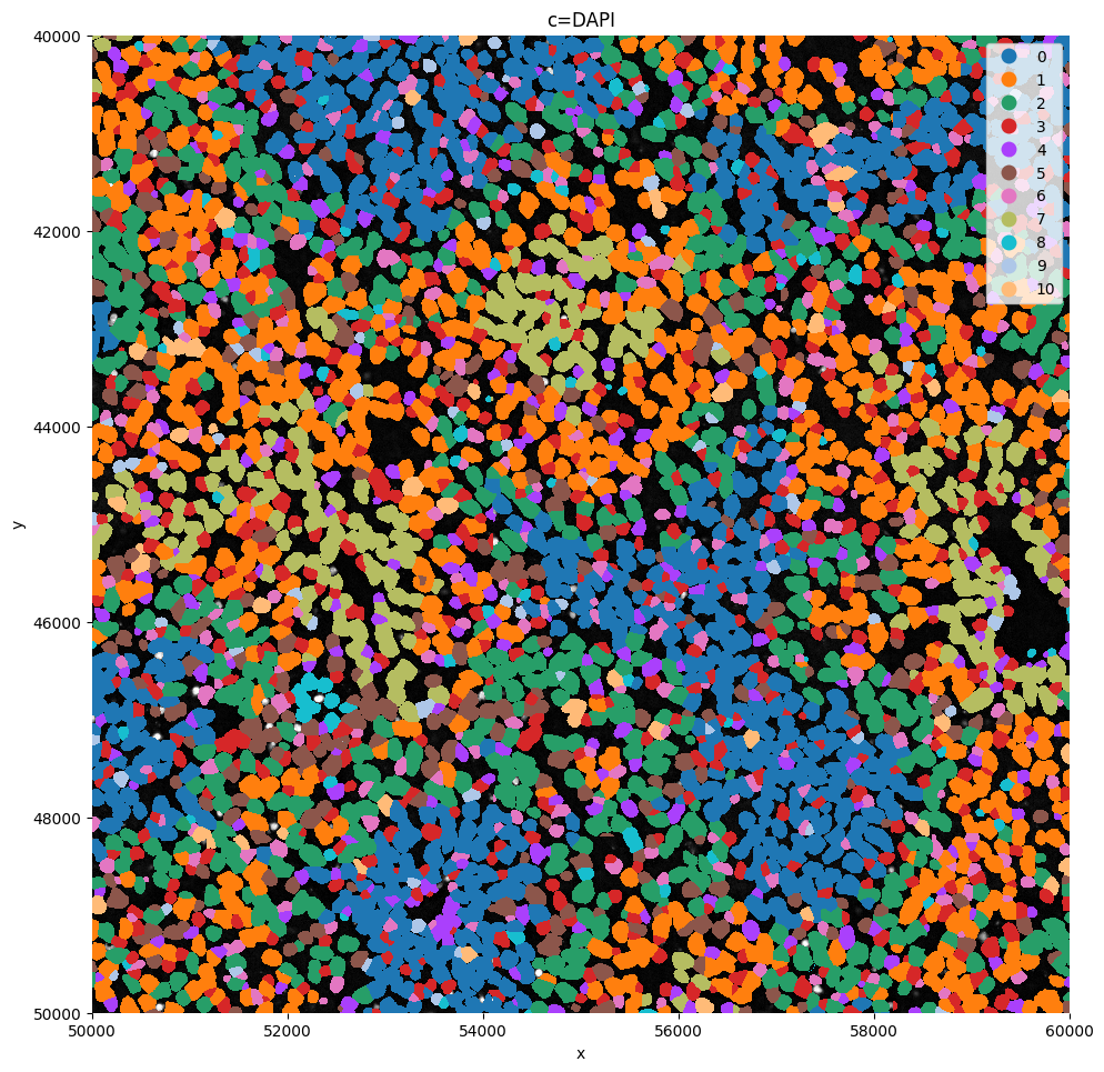
sp.pl.plot_shapes(
    sdata,
    img_layer="clahe",
    table_layer="table_transcriptomics_clustered_crop",
    column="leiden",
    shapes_layer="segmentation_mask_boundaries_crop",
    alpha=1,
    linewidth=0,
    channel="DAPI",
    crd = [ 50000, 60000, 40000, 50000 ],
)
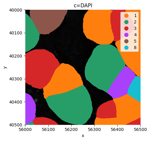
Or visualize a crop.
sp.pl.plot_shapes(
    sdata,
    img_layer="clahe",
    table_layer="table_transcriptomics_clustered_crop",
    column="leiden",
    shapes_layer="segmentation_mask_boundaries_crop",
    alpha=1,
    linewidth=0,
    channel="DAPI",
    crd = [ 56000, 56000+500, 40000, 40500 ],
    figsize=(5,5),
)